Circuit Theorems

Linearity Property

Linear property is the linear relationship between cause and effect of an element. This property gives linear and nonlinear circuit definition. The property can be applied in various circuit elements. The homogeneity property and the additivity property are both the combination of linearity property.

The homogeneity property is that if the input is multiplied by a constant k then the output is also multiplied by the constant k. Input is called excitation and output is called response here. As an example if we consider ohm’s law. Here the law relates the input i to the output v. 

Mathematically,                                      v= iR

If we multiply the input current  i by a constant k then the output voltage also increases correspondingly by the constant k. The equation stands, 

                                                            kiR = kv

The additivity property is that the response to a sum of inputs is the sum of the responses to each input applied separately.

Using voltage-current relationship of a resistor if

                                                  v₁ = i₁R       and   v₂ = i₂R

Applying (i₁ + i₂)gives

 

                                              V = (i₁ + i₂)R = i₁R+ i₂R = v₁ + v₂

We can say that a resistor is a linear element. Because the voltage-current relationship satisfies both the additivity and the homogeneity properties.

We can tell a circuit is linear if the circuit both the additive and the homogeneous. A linear circuit always consists of linear elements, linear independent and dependent sources.

 Linearity Circuit

A linear circuit is one whose output is linearly related (or directly proportional) to its input.

A linear circuit is a special system whose output is linearly related. Linear circuits are very useful in modeling devices and very well understood. 

To learn more about Linearity:

SUPERPOSITION

• The superposition theorem eliminates the need for solving simultaneous linear equations by considering the effect on each source independently.

•  To consider the effects of each source we remove the remaining sources; by setting the voltage sources to zero (short-circuit representation) and current sources to zero (open-circuit representation).

•  The current through, or voltage across, a portion of the network produced by each source is then added algebraically to find the total solution for current or voltage.

•  The only variation in applying the superposition theorem to AC networks with independent sources is that we will be working with impedances and phasors instead of just resistors and real numbers.

•   The superposition theorem is not applicable to power effects in AC networks since we are still dealing with a nonlinear relationship.

•  It can be applied to networks with sources of different frequencies only if the total response for each frequency is found independently and the results are expanded in a nonsinusoidal expression.

•  One of the most frequent applications of the superposition theorem is to electronic systems in which the DC and AC analyses are treated separately and the total solution is the sum of the two.

 

When a circuit has sources operating at different frequencies, the separate phasor circuit for each frequency must be solved independently, and the total response is the sum of time-domain responses of all the individual phasor circuits. Superposition Theorem applies to AC circuits as well. For sources having different frequencies, the total response must be obtained by adding individual responses in time domain.



These are some Superposition Technique for sources having different frequencies.

All sources except DC 5-V set to zero

  All sources except 10cos(10t) set to zero

All sources except 2 sin 5t set to zero

vo= v1+ v2+ v3

Consider the following example:

The principle of superposition helps us to analyze a linear circuit with more than one independent source by calculating the contribution of each independent source separately. However, to apply the superposition
principle, we must keep two things in mind:


1. We consider one independent source at a time while all other independent sources are turned off. This implies that we replace every voltage source by 0 V (or a short circuit), and every current source by 0 A (or an open circuit). This way we obtain a simpler and more manageable circuit.

2. Dependent sources are left intact because they are controlled by circuit variables. With these in mind, we apply the superposition principle in three steps.


 Steps to Apply Superposition Principle:
 
1. Turn off all independent sources except one source.

2. Repeat step 1 for each of the other independent sources.

3. Find the total contribution by adding algebraically all the contributions due to the independent sources.

 SUPERPOSITION

Transform a voltage source in series with impedance to a current source in parallel with impedance for simplification or vice versa.

Consider the following example: Calculate the current Io.

  

If we transform the current source to a voltage source, we obtain the circuit shown in Fig. (a).

By current division,

A source transformation is the process of replacing a voltage source vs in series with a resistor R by a current source is in parallel with a resistor R, or vice versa.

Voltage Source Transformation

 We will first go over voltage source transformation, the transformation of a circuit with a voltage source to the equivalent circuit with a current source. In order to get a visual example of this, let's take the circuit below which has a voltage source as its power source:

Using source transformation, we can change or transform this above circuit with a voltage power source and a resistor, R, in series, into the equivalent circuit with a current source with a resistor, R, in parallel, as shown below:
 

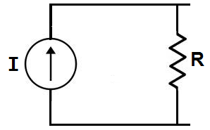
We transform a voltage source into a current source by using ohm's law. A voltage source can be changed into a current source by using ohm's formula, I=V/R.

Current Source Transformation

We will now go over current source transformation, the transformation of a circuit with a current source to the equivalent circuit with a voltage source. In order to get a visual example of this, let's take the circuit below which has a current source as its power source:

Using source transformation, we can change or transform this above circuit with a current power source and a resistor, R, in parallel, into the equivalent circuit with a voltage source with a resistor, R, in series, as shown below:

We transform a current source into a voltage source by using ohm's law. A voltage source can be changed into a current source by using ohm's formula, V= IR. 

 

 

TO KNOW MORE ABOUT SOURCE TRANSFORMATION:

 

 

MESH ANALYSIS

Mesh Analysis

Mesh analysis is a method that is used to solve planar circuits for the currents  at any place in the circuit. Planar circuits are circuits that can be drawn on a plane surface with no wires crossing each other. Mesh analysis use Kirchhoff’s voltage law to arrive at a set of equations guaranteed to be solvable if the circuit has a solution.

Using mesh currents instead of element currents as circuit variables is convenient and reduces the number of
equations that must be solved simultaneously. Recall that a loop is a closed path with no node passed more than once. A mesh is a loop that does not contain any other loop within it.

A mesh is a loop which does not contain any other loops within it.

Steps to Determine Mesh Currents:

1. Assign mesh currents to the n meshes.

2. Apply KVL to each of the n meshes. Use Ohm’s law to express the voltages in terms of the mesh currents.

3. Solve the resulting n simultaneous equations to get the mesh currents.

Mesh Analysis with Current Sources

Two possible cases:

• CASE 1 : When a current source exists only in one mesh.

• CASE 2 : When a current source exists between two meshes:  We create a SUPERMESH by excluding the current source and any elements connected in series with it.

A supermesh results when two meshes have a (dependent or independent) current source in common.

Nodal Analysis with Voltage Source

Nodal Analysis with Voltage Source 

Nodal analysis is the method to determine voltage or current using nodes of the circuit. In nodal analysis we choose node voltage instead of element voltages and hence the equations reduces in this process. We have to consider voltage source is not in this circuit. We have to solve a circuit with n nodes without voltage sources. To solve a circuit using nodal analysis method you must have good knowledge about node branch loop in a circuit.

Two cases:

• Case 1: If a voltage source is connected between the reference node and a non-reference node, we simply set the voltage at the non-reference node equal to the voltage of the voltage source.

• CASE 2: If the voltage source (dependent or independent) is connected between two non-reference nodes, the two non-reference nodes form a Super Node. Apply KCL and KVL to determine the node voltages.

#Super node is formed by enclosing a (dependent or independent) voltage source connected between two non-reference nodes and any elements connected in parallel with it.

Properties of Super Node:

1. The voltage source inside the super node provides a constraint equation needed to solve for the node voltages.
2. A super node has no voltage of its own.
3. A super node requires the application of both KCL and KVL.
   
   
   
   
   In figure 2,  Apply the KCL at super node which are node 2 and 3 we get,
                                           i₁ + i₄  = i₂ + i₃
   
   To apply KVL redrawing the figure 2 circuit to figure 3 and going around the loop in the clockwise direction gives,
                          – v₂ + 10 + v₃ = 0
                           Or  v₂ – v₃ = 10      ————————— (ii)
   From equation (i),(ii) we will obtain node voltages using any solution method.

Nodal Analysis

What is Nodal Analysis?

Nodal analysis provides a general procedure for analyzing circuits using node voltages as the circuit variables.

In electric circuits analysis, nodal analysis, node-voltage analysis, or the branch current method is a method of determining the voltage (potential difference) between "nodes" (points where elements or branches connect) in an electrical circuit in terms of the branch currents.

By using Kirchhoff's circuit laws, one can either do nodal analysis using Kirchhoff's current law (KCL) or mesh analysis using Kirchhoff's voltage law (KVL). 

For instance, for a resistor, I_branch = V_branch * G, where G (=1/R) is the admittance (conductance) of the resistor.

 Nodal analysis produces a compact set of equations for the network, which can be solved by hand if small, or can be quickly solved using linear algebra by computer.

While simple examples of nodal analysis focus on linear elements, more complex nonlinear networks can also be solved with nodal analysis by using Newton's method to turn the nonlinear problem into a sequence of linear problems.

In nodal analysis, we are about to find the node voltages. Given a circuit with n nodes without voltage sources, the nodal analysis of the circuit involves taking the following steps:

1. Select a node as the reference node. Assign voltages to the remaining nodes. The voltages are referenced with respect to the reference node. 
2. Apply KCL to each of the n-1 non-reference nodes. Use Ohm’s law to express the branch currents in terms of node voltages.
3. Solve the resulting simultaneous equations to obtain the unknown node voltages.
    
   Current flows from a HIGHER POTENTIAL to a LOWER POTENTIAL in a resistor.

i = vhigher - vlower / R

Some Example of Wye Delta

EXAMPLE PROBLEM OF WYE TO DELTA TRANSFORMATION 

Find the resistance shown by the meter !

Let's convert the R₁, R₂, R₃ wye network to a delta network. This conversion is the best choice for simplifying this network.

First, we do the Wye to delta conversion, then we notice the instances of paralleled resistors in the simplified circuit.

{Wye to delta conversion for R1, R2, R3 }

Gy: = 1/R1+1/R2+1/R3;

Gy = [95m]

RA =R1*R2*Gy;

RB =R1*R3*Gy;

RC=R2*R3*Gy;

Req:=Re-plus (Re-plus(R6,RB), (Re-plus(R4,RA)+Re-plus(R5,RC)));

RA=[76]

RB=[95]

RC=[190]

Req=[35]

EXAMPLE PROBLEM OF DELTA TO WYE TRANSFORMATION

Here we go through an example that utilizes a delta to wye transformation, along with series and parallel resistance equations.